Introduction • roams

In this vignette, we provide a summary of the main R functions contained in the roams package and how to use them. We’ll begin by simulating a data set, fitting a model, inspecting results, and finally using the model to perform out-of-sample (OOS) filtering.

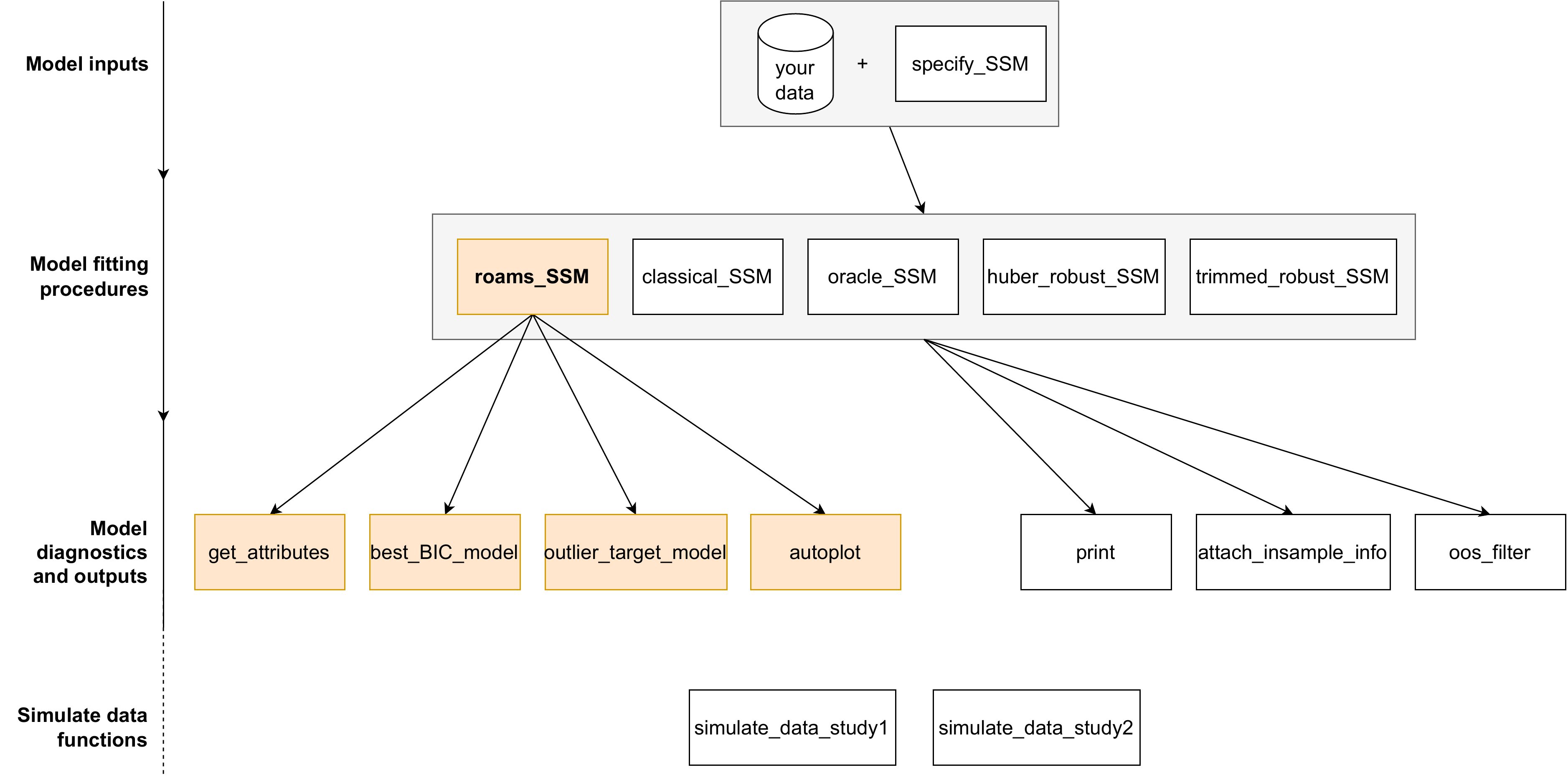
Overview of roams functions

We start by loading the required packages and setting a simple ggplot2 theme for consistent plotting.

library(roams)
library(tidyverse)
library(patchwork)

theme_set(
  theme_bw(base_size = 14) + 
    theme(legend.position = "bottom",
          legend.key.width = unit(1.2, "cm"))
)

Simulating data

roams provides a helper function simulate_data_study1() which generates example data sets used in the simulations results of Study 1 in Shankar et al. (2025). We use this function to simulate a single sample (samples = 1) for each of the different sample sizes and outlier settings, and extract specifically the cluster setting with $n=100$ timepoints.

data = simulate_data_study1(samples = 1, seed = 12345) |> 
  filter(n == 100, setting == "cluster")

The data set contains a column y which contains an observation in each row:

y = data$y[[1]]
head(y)
#>             [,1]        [,2]
#> [1,]  1.21665121  0.01718996
#> [2,]  0.03387945  1.43366185
#> [3,] -0.07748398  0.72068394
#> [4,] 20.07176363 18.22658579
#> [5,] -0.13745034  2.26740843
#> [6,]  1.06648254  2.27373266

As you can see, the observations are 2-dimensional. You can think of each observation as a longitude/latitude coordinate of an object moving through 2D space. We can plot these observations indexed by time:

plot_data = tibble(
  y1 = y[,1],
  y2 = y[,2],
  timepoint = 1:100
) 

ggplot(plot_data) +
  aes(x = y1, y = y2, colour = timepoint) +
  geom_point() +
  scale_colour_viridis_c()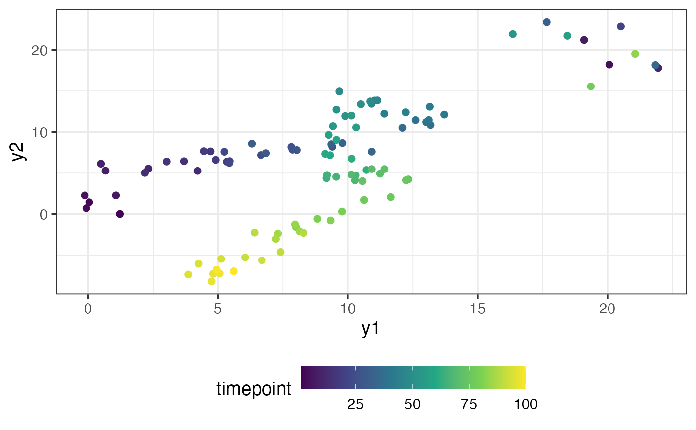

The object first starts near the coordinate $[0,0]$ , then it moves in the positive $[y_1, y_2]$ direction, and then it loops around before moving back in the the negative $[y_1, y_2]$ direction. In the top right, there are a few observations scattered away from the main trajectory taken by the object. We suspect that these points are outliers.

Fitting a ROAMS state-space model

Here are the state and observation equations for a linear Gaussian state-space model:

$\begin{align} \boldsymbol y_t &= \boldsymbol A \boldsymbol x_t + \boldsymbol v_t \\ \boldsymbol x_t &= \boldsymbol \Phi \boldsymbol x_{t-1} + \boldsymbol w_t, \end{align}$

where $\boldsymbol y_t$ is the observation process, $\boldsymbol x_t$ is the state process, $\boldsymbol v_t \sim N(\boldsymbol 0, \boldsymbol\Sigma_{\boldsymbol v})$ and $\boldsymbol w_t \sim N(\boldsymbol 0, \boldsymbol\Sigma_{\boldsymbol w})$ . The state-space model we want to use to model our data is the first-differenced correlated random walk (DCRW) model. The DCRW model has a 2-dimensional $\boldsymbol y_t$ and a 4-dimensional $\boldsymbol x_t$ because $\boldsymbol x_t$ tries to capture the true location of the object at times $t$ and $t-1$ (see Shankar et al. (2025) for more details). The matrices in the DCRW model are given by

$\begin{align} \boldsymbol\Phi &= \left[ \begin{matrix} 1+\phi&0&-\phi&0 \\ 0&1+\phi&0&-\phi \\ 1&0&0&0 \\ 0&1&0&0 \\ \end{matrix} \right] \\ \boldsymbol A &= \left[ \begin{matrix} 1&0&0&0 \\ 0&1&0&0 \end{matrix} \right], \end{align}$

and the error variance matrices are $\boldsymbol\Sigma_{\boldsymbol v} = \text{diag}(\sigma^2_{\boldsymbol v,1}, \sigma^2_{\boldsymbol v,2})$ and $\boldsymbol\Sigma_{\boldsymbol w} = \text{diag}(\sigma^2_{\boldsymbol w,1}, \sigma^2_{\boldsymbol w,2}, 0, 0)$ . We assume at time $t=0$ , that $\boldsymbol x_0 \sim N(\boldsymbol\mu_0, \boldsymbol P_0)$ , where $\boldsymbol\mu_0 = [0,0,0,0]$ and $\boldsymbol P_0 = \text{diag}(10^2, 10^2, 10^2, 10^2)$ .

There are a total of 5 unknown parameters in the DCRW model: $\boldsymbol\theta := [\phi,\sigma^2_{\boldsymbol w,1}, \sigma^2_{\boldsymbol w,2}, \sigma^2_{\boldsymbol v,1}, \sigma^2_{\boldsymbol v,2}]$ . To specify this model, we define a function build_fn() that takes in $\boldsymbol\theta$ as an argument and returns $\boldsymbol x_0, \boldsymbol P_0, \boldsymbol\Phi, \boldsymbol A, \boldsymbol\Sigma_{\boldsymbol v}, \boldsymbol\Sigma_{\boldsymbol w}$ . The helper function specify_SSM() is used inside build_fn() to help return these values in the correct format.

build_fn = function(par) {
  
  phi_coef = par[1]
  Phi = diag(c(1+phi_coef, 1+phi_coef, 0, 0))
  Phi[1,3] = -phi_coef
  Phi[2,4] = -phi_coef
  Phi[3,1] = 1
  Phi[4,2] = 1
  
  A = diag(4)[1:2,]
  Sigma_w = diag(c(par[2], par[3], 0, 0))
  Sigma_v = diag(c(par[4], par[5]))
  
  mu0 = c(0,0,0,0)
  P0 = diag(rep(10^2, 4))
  
  specify_SSM(
    state_transition_matrix = Phi,
    state_noise_var = Sigma_w,
    observation_matrix = A,
    observation_noise_var = Sigma_v,
    init_state_mean = mu0,
    init_state_var = P0)
}

To fit the model using the ROAMS procedure, we use the function roams_SSM() and pass in the observations y as well as our model specification function build_fn(). Since $\phi \in[0,1]$ and $\sigma^2_{\boldsymbol w,1}, \sigma^2_{\boldsymbol w,2}, \sigma^2_{\boldsymbol v,1}, \sigma^2_{\boldsymbol v,2} > 0$ , we add in these parameter box constraints via the lower and upper arguments. We provide initial parameter values $[0.5, 1, 1, 1, 1]$ and we set num_lambdas = 20 to let roams_SSM() automatically select a sequence of 20 $\lambda$ values to fit candidate models.

model_list = roams_SSM(
  y = y, 
  init_par = c(0.5, rep(1, 4)), 
  build = build_fn, 
  num_lambdas = 20, 
  lower = c(0, rep(1e-12, 4)), 
  upper = c(1, rep(Inf, 4))
)

model_list
#> ROAMS SSM List with 20 models
#>  * Use best_BIC_model() or outlier_target_model() to extract a preferred model.
#>    - Or, simply use list indexing such as [[1]] to extract a single model.
#>  * Use autoplot() to visualize the models.
#>  * Use get_attribute() to extract attributes from the models.

Inspecting the models

Once the models have been fit and assigned to the variable model_list, we can plot BIC and proportion-outlying curves across the values of $\lambda$ using the autoplot() function:

autoplot(model_list)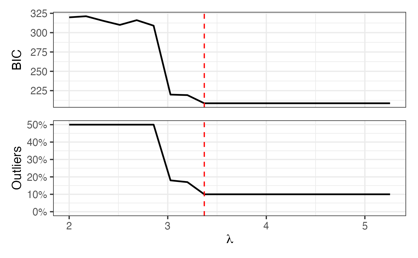

The exact BIC or proportion-outlying values can be obtained using the get_attribute() function:

get_attribute(model_list, "prop_outlying")
#>  [1] 0.50 0.50 0.50 0.50 0.50 0.50 0.18 0.17 0.10 0.10 0.10 0.10 0.10 0.10 0.10
#> [16] 0.10 0.10 0.10 0.10 0.10

To extract the model corresponding to the lowest BIC, we can use the best_BIC_model() function. We assign this model to the variable final_model:

final_model = best_BIC_model(model_list)
final_model
#> ROAMS SSM Model
#>  * Lambda: 3.371
#>  * Outliers Detected: 10%
#>  * BIC: 208.663
#>  * Log-Likelihood: -81.306
#>  * Iterations: 6
#> Use $ to see more attributes.

As shown above, printing final_model provides a brief summary of the model. It tells us which $\lambda$ value was selected, the proportion of timepoints detected as outlying, the BIC, log-likelihood, and the number of ROAMS iterations.

Other model-specific attributes such as par (parameter estimates) can be viewed using $:

final_model$par
#> [1] 0.5522448 0.1655666 0.2131430 0.3093632 0.2475860

By default, more detailed information such as estimates for the hidden states are not included in the model object to save memory. However, we need this information to plot the estimated states. To get this information, we can use the attach_insample_info() function:

final_model = attach_insample_info(final_model)

Below, we use our final_model to plot the `smoothed’ estimated trajectory of the moving object as well as circle the observations detected as outliers in red.

outliers = rowSums(abs(final_model$gamma)) != 0

plot_data = tibble(
  y1 = y[,1],
  y2 = y[,2],
  y1_model = final_model$smoothed_observations[,1],
  y2_model = final_model$smoothed_observations[,2],
  outliers = outliers,
  timepoint = 1:100
)

ggplot(plot_data) +
  aes(x = y1, y = y2, colour = timepoint) +
  geom_point(alpha = 0.3) +
  geom_path(aes(x = y1_model, y = y2_model), 
            linewidth = 1) +
  geom_point(data = plot_data |> filter(outliers),
             colour = "red", pch = 1) +
  scale_colour_viridis_c()

The fit looks good and the suspected outliers have been correctly detected.

Out-of-sample (OOS) filtering

The simulated data set that we generated contains another column named y_oos, which contains $n_{\text{oos}} = 20$ out-of-sample observations. We will use our final_model to obtain filtered values for y_oos.

The out-of-sample data has the same characteristics as the in-sample data, except that it starts where the in-sample data ends. We re-define our build_fn() to set the initial state mean $\boldsymbol\mu_0$ to be our best guess of the hidden state at the last in-sample timepoint, $t=100$ :

final_model$smoothed_states[100,]
#> [1]  5.374293 -6.914360  5.149415 -7.047400

y_oos = data$y_oos[[1]]

build_fn_oos = function(par) {
  
  phi_coef = par[1]
  Phi = diag(c(1+phi_coef, 1+phi_coef, 0, 0))
  Phi[1,3] = -phi_coef
  Phi[2,4] = -phi_coef
  Phi[3,1] = 1
  Phi[4,2] = 1
  
  A = diag(4)[1:2,]
  Sigma_w = diag(c(par[2], par[3], 0, 0))
  Sigma_v = diag(c(par[4], par[5]))
  
  mu0 = final_model$smoothed_states[100,]
  P0 = diag(rep(10^2, 4))
  
  specify_SSM(
    state_transition_matrix = Phi,
    state_noise_var = Sigma_w,
    observation_matrix = A,
    observation_noise_var = Sigma_v,
    init_state_mean = mu0,
    init_state_var = P0)
}

Using this new state-space model specification, build_fn_oos, we can do out-of-sample filtering using the oos_filter() function. We supply data y_oos, the model final_model (which is needed for its parameter estimates), and our function build_fn_oos:

result = oos_filter(y_oos, final_model, build_fn_oos)

head(result$filtered_observations)
#>          [,1]       [,2]
#> [1,] 6.388546  -8.246328
#> [2,] 8.072338  -6.445772
#> [3,] 8.755492  -7.236791
#> [4,] 8.457210  -8.312808
#> [5,] 9.388451  -9.028853
#> [6,] 9.743224 -10.004715

Below, we plot the out-of-sample observations alongside our filtered values. The fit is pretty good:

plot_data = tibble(
  y1 = y_oos[,1],
  y2 = y_oos[,2],
  y1_filter = result$filtered_observations[,1],
  y2_filter = result$filtered_observations[,2],
  timepoint = 1:20
)

ggplot(plot_data) +
  aes(x = y1, y = y2, colour = timepoint) +
  geom_point(alpha = 0.3) +
  geom_path(aes(x = y1_filter, y = y2_filter), 
            linewidth = 1) +
  scale_colour_viridis_c()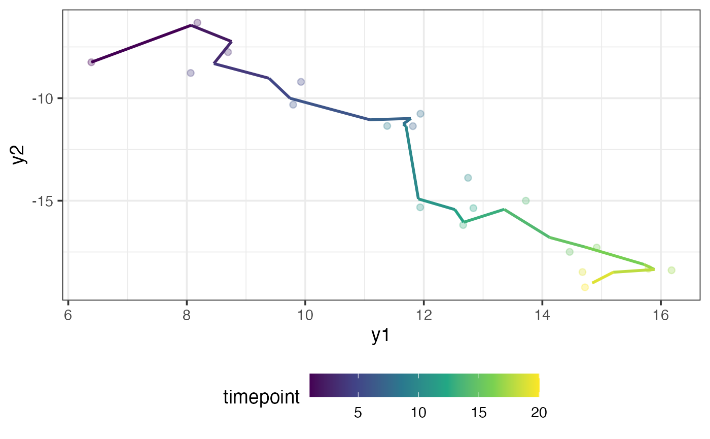

Notice that there are no visible outliers in the out-of-sample data. Let’s see what happens to our filtered values if there is an outlier. We can contaminate the 10 $^\text{th}$ observation to be outlying:

y_oos[10,] = y_oos[10,] + c(10,10)
y_oos[10,]
#> [1] 22.746904 -3.882899

If the model passed to oos_filter() is of class roams_SSM, then by default the oos_filter() function uses the fast-updating threshold (FUT) filter (see Shankar et al. (2025)) to do out-of-sample filtering. The FUT filter provides robustness against out-of-sample outliers. If the usual Kalman filter is desired, we can set the argument threshold = Inf. We try both filters:

result_FUT = oos_filter(y_oos, final_model, build_fn_oos)
result_kalman = oos_filter(y_oos, final_model, build_fn_oos, threshold = Inf)

Below, we plot the filtered values against the out-of-sample data (where the 10 $^\text{th}$ point has been contaminated) for both filtering methods:

plot_data = tibble(
  y1 = y_oos[,1],
  y2 = y_oos[,2],
  y1_FUT = result_FUT$filtered_observations[,1],
  y2_FUT = result_FUT$filtered_observations[,2],
  y1_kalman = result_kalman$filtered_observations[,1],
  y2_kalman = result_kalman$filtered_observations[,2],
  timepoint = 1:20
)

p_FUT = ggplot(plot_data) +
  aes(x = y1, y = y2, colour = timepoint) +
  geom_point(alpha = 0.3) +
  geom_path(aes(x = y1_FUT, y = y2_FUT), 
            linewidth = 1) +
  ggtitle("FUT") +
  scale_colour_viridis_c()

p_kalman = ggplot(plot_data) +
  aes(x = y1, y = y2, colour = timepoint) +
  geom_point(alpha = 0.3) +
  geom_path(aes(x = y1_kalman, y = y2_kalman), 
            linewidth = 1) +
  ggtitle("Kalman") +
  scale_colour_viridis_c()

p_FUT + p_kalman + plot_layout(guides = "collect", axes = "collect")

As you can see, the FUT filter is able to ignore the outlier whereas the Kalman filter gets pulled towards it.

Summary

In this vignette, we demonstrated the core functionality of the roams package through a complete end-to-end example. We began by simulating bivariate time series data using simulate_data_study1(), then specified a state-space model (the DCRW model) through the helper function specify_SSM(). Using roams_SSM(), we fitted a sequence of models across different values of the tuning parameter $\lambda$ and identified the optimal model via the BIC criterion.

We then explored how to inspect fitted models, extract key quantities (such as parameter estimates and detected outliers), and visualise model diagnostics using autoplot() and smoothed states using attach_insample_info().

Finally, we illustrated how to use the fitted model for out-of-sample (OOS) filtering, showing that the fast-updating threshold (FUT) filter can effectively resist the influence of outliers compared to the standard Kalman filter.

References

Shankar, R., Wilms, I., Raymaekers, J., & Tarr, G. (2025). Robust outlier-adjusted mean-shift estimation of state-space models. https://arxiv.org/abs/????.?????