Simulation study 2

This page shows how the simulation results in Section 4.2 of Shankar et al. (2025) are generated.

library(tidyverse)
library(roams) # version 0.6.5
library(future)

## Number of cores to use
num_cores = 8
study = "study2"
seed = paste0("seed", 2025.2)
data_path = "data/"
scripts_path = "scripts/"
run_sim = FALSE

Simulate data for Study 2

true_par = c(0.8, 0.1, 0.1, 0.4, 0.4)

data_study2 = simulate_data_study2(
  samples = 200,  # change to 200?
  n = 200,
  max_contamination = 0.2,
  distances = c(1, 3, 5, 7, 9),
  n_oos = 20,
  phi_coef = true_par[1],
  sigma2_w_lon = true_par[2],
  sigma2_w_lat = true_par[3],
  sigma2_v_lon = true_par[4],
  sigma2_v_lat = true_par[5],
  initial_state = c(0, 0, 0, 0),
  seed = as.numeric(str_remove(seed, "seed"))
)

readr::write_rds(data_study2, 
                 paste0(data_path, "data_", study, "_", seed, ".rds"))

Fit models for Study 2

5 models are fit to each data set: classical, oracle, ROAMS, Huber, and trimmed. Each data frame of models can be large in size and takes days to fit, so they are saved in 5 separate .rds files.

• Classical SSM fit
• Oracle model
• ROAMS
• Huber model
• Trimmed model

plan(multisession, workers = num_cores)
classical_start = Sys.time()
model_fits_classical_study2 = data_study2 |> 
  mutate(
    classical_model = furrr::future_map(y, function(y) {
      
      build = function(par) {
    
        phi_coef = par[1]
        Phi = diag(c(1+phi_coef, 1+phi_coef, 0, 0))
        Phi[1,3] = -phi_coef
        Phi[2,4] = -phi_coef
        Phi[3,1] = 1
        Phi[4,2] = 1
        
        A = diag(4)[1:2,]
        Q = diag(c(par[2], par[3], 0, 0))
        R = diag(c(par[4], par[5]))
        
        x0 = c(y[1,], y[1,])
        P0 = diag(rep(0, 4))
        
        specify_SSM(
          state_transition_matrix = Phi,
          state_noise_var = Q,
          observation_matrix = A,
          observation_noise_var = R,
          init_state_mean = x0,
          init_state_var = P0)
      }
      
      classical_SSM(
        y = y, 
        init_par = c(0.5, rep(c(mad(diff(y[,1]), na.rm = TRUE)^2, 
                                mad(diff(y[,2]), na.rm = TRUE)^2), 2)),
        build = build, 
        lower = c(0, rep(1e-12, 4)), 
        upper = c(1, rep(Inf, 4))
      )}, 
    .progress = TRUE),
    .keep = "none")
classical_end = Sys.time()
classical_end - classical_start
readr::write_rds(model_fits_classical_study2, 
                 paste0(data_path, "classical_", study, "_", seed, ".rds"), 
                 compress = "gz")
plan(sequential)
rm(model_fits_classical_study2)  ## free up memory

plan(multisession, workers = num_cores)
oracle_start = Sys.time()
model_fits_oracle_study2 = data_study2 |> 
  mutate(
    oracle_model = furrr::future_map2(y, outlier_locs, function(y, outlier_locs) {
      
      build = function(par) {
    
        phi_coef = par[1]
        Phi = diag(c(1+phi_coef, 1+phi_coef, 0, 0))
        Phi[1,3] = -phi_coef
        Phi[2,4] = -phi_coef
        Phi[3,1] = 1
        Phi[4,2] = 1
        
        A = diag(4)[1:2,]
        Q = diag(c(par[2], par[3], 0, 0))
        R = diag(c(par[4], par[5]))
        
        x0 = c(y[1,], y[1,])
        P0 = diag(rep(0, 4))
        
        specify_SSM(
          state_transition_matrix = Phi,
          state_noise_var = Q,
          observation_matrix = A,
          observation_noise_var = R,
          init_state_mean = x0,
          init_state_var = P0)
      }
      
      oracle_SSM(
        y = y,
        init_par = c(0.5, rep(c(mad(diff(y[,1]), na.rm = TRUE)^2, 
                                mad(diff(y[,2]), na.rm = TRUE)^2), 2)),
        build = build, 
        outlier_locs = outlier_locs,
        lower = c(0, rep(1e-12, 4)), 
        upper = c(1, rep(Inf, 4))
      )}, 
    .progress = TRUE),
    .keep = "none")
oracle_end = Sys.time()
oracle_end - oracle_start
readr::write_rds(model_fits_oracle_study2, 
                 paste0(data_path, "oracle_", study, "_", seed, ".rds"),
                 compress = "gz")
plan(sequential)
rm(model_fits_oracle_study2)  ## free up memory

plan(multisession, workers = num_cores)

roams_start = Sys.time()
model_fits_roams_study2 = data_study2 |> 
  mutate(
    model_list = furrr::future_map(y, function(y) {
      
      build = function(par) {
    
        phi_coef = par[1]
        Phi = diag(c(1+phi_coef, 1+phi_coef, 0, 0))
        Phi[1,3] = -phi_coef
        Phi[2,4] = -phi_coef
        Phi[3,1] = 1
        Phi[4,2] = 1
        
        A = diag(4)[1:2,]
        Q = diag(c(par[2], par[3], 0, 0))
        R = diag(c(par[4], par[5]))
        
        x0 = c(y[1,], y[1,])
        P0 = diag(rep(0, 4))
        
        specify_SSM(
          state_transition_matrix = Phi,
          state_noise_var = Q,
          observation_matrix = A,
          observation_noise_var = R,
          init_state_mean = x0,
          init_state_var = P0)
      }
      
      roams_SSM(
        y = y, 
        init_par = c(0.5, rep(c(mad(diff(y[,1]), na.rm = TRUE)^2, 
                                mad(diff(y[,2]), na.rm = TRUE)^2), 2)), 
        build = build, 
        num_lambdas = 20, 
        cores = 1,
        lower = c(0, rep(1e-12, 4)), 
        upper = c(1, rep(Inf, 4)),
        B = 50
      )}, 
    .progress = TRUE),
    best_BIC_model = map(model_list, best_BIC_model),
    .keep = "none")
roams_end = Sys.time()
roams_end - roams_start
readr::write_rds(model_fits_roams_study2, 
                 paste0(data_path, "roams_", study, "_", seed, ".rds"), 
                 compress = "gz")
plan(sequential)
rm(model_fits_roams_study2)  ## free up memory

plan(multisession, workers = num_cores)
huber_start = Sys.time()
model_fits_huber_study2 = data_study2 |>
  mutate(
    huber_model = furrr::future_map(y, function(y) {
      
      build_huber_trimmed = function(par) {
    
        phi_coef = par[1]
        Phi = diag(c(1+phi_coef, 1+phi_coef, 0, 0))
        Phi[1,3] = -phi_coef
        Phi[2,4] = -phi_coef
        Phi[3,1] = 1
        Phi[4,2] = 1
      
        A = diag(4)[1:2,]
        Q = diag(c(par[2], par[3], 0, 0))
        R = diag(c(par[4], par[5]))
        
        x0 = c(y[1,], y[1,] + 0.01)
        P0 = diag(rep(0, 4))
        
        specify_SSM(
          state_transition_matrix = Phi,
          state_noise_var = Q,
          observation_matrix = A,
          observation_noise_var = R,
          init_state_mean = x0,
          init_state_var = P0)
      }
      
      huber_robust_SSM(
        y = y,
        init_par = c(0.5, rep(c(mad(diff(y[,1]), na.rm = TRUE)^2, 
                                mad(diff(y[,2]), na.rm = TRUE)^2), 2)),
        build = build_huber_trimmed,
        lower = c(0.001, rep(1e-12, 4)),
        upper = c(0.999, rep(Inf, 4))
      )},
    .progress = TRUE),
    .keep = "none")
huber_end = Sys.time()
huber_end - huber_start
readr::write_rds(model_fits_huber_study2, 
                 paste0(data_path, "huber_", study, "_", seed, ".rds"), 
                 compress = "gz")
plan(sequential)
rm(model_fits_huber_study2)  ## free up memory

plan(multisession, workers = num_cores)
trimmed_start = Sys.time()
model_fits_trimmed_study2 = data_study2 |>
  mutate(
    trimmed_model = furrr::future_map2(y, contamination, 
                                       function(y, contamination) {
      
      build_huber_trimmed = function(par) {
    
        phi_coef = par[1]
        Phi = diag(c(1+phi_coef, 1+phi_coef, 0, 0))
        Phi[1,3] = -phi_coef
        Phi[2,4] = -phi_coef
        Phi[3,1] = 1
        Phi[4,2] = 1
      
        A = diag(4)[1:2,]
        Q = diag(c(par[2], par[3], 0, 0))
        R = diag(c(par[4], par[5]))
        
        x0 = c(y[1,], y[1,] + 0.01)
        P0 = diag(rep(0, 4))
        
        specify_SSM(
          state_transition_matrix = Phi,
          state_noise_var = Q,
          observation_matrix = A,
          observation_noise_var = R,
          init_state_mean = x0,
          init_state_var = P0)
      }
      
      trimmed_robust_SSM(
        y = y,
        init_par = c(0.5, rep(c(mad(diff(y[,1]), na.rm = TRUE)^2, 
                                mad(diff(y[,2]), na.rm = TRUE)^2), 2)),
        build = build_huber_trimmed,
        alpha = contamination,
        lower = c(0.001, rep(1e-12, 4)),
        upper = c(0.999, rep(Inf, 4))
      )},
    .progress = TRUE),
    .keep = "none")
trimmed_end = Sys.time()
trimmed_end - trimmed_start
readr::write_rds(model_fits_trimmed_study2,
                 paste0(data_path, "trimmed_", study, "_", seed, ".rds"),
                 compress = "gz")
plan(sequential)
rm(model_fits_trimmed_study2)  ## free up memory

Compute evaluation metrics for fitted models

Using the model fits, in-sample and out-of-sample evaluation metrics (sensitivity, specificity, estimation RMSE, one-step-ahead MSFE) are computed. Functions to compute these metrics are sourced from the scripts/evaluation_functions.R script file. This process takes a few minutes to run, so the output is saved to the file data/eval_metrics_study2.rds.

classical_study2 = read_rds(paste0(
  data_path, "classical_", study, "_", seed, ".rds"))
roams_study2 = read_rds(paste0(
  data_path, "roams_", study, "_", seed, ".rds"))
oracle_study2 = read_rds(paste0(
  data_path, "oracle_", study, "_", seed, ".rds"))
huber_study2 = read_rds(paste0(
  data_path, "huber_", study, "_", seed, ".rds"))
trimmed_study2 = read_rds(paste0(
  data_path, "trimmed_", study, "_", seed, ".rds"))

data_study2 = read_rds(paste0(
  data_path, "data_", study, "_", seed, ".rds"))
model_fits_study2 = data_study2 |> 
  bind_cols(classical_study2) |> 
  bind_cols(roams_study2) |> 
  bind_cols(oracle_study2) |> 
  bind_cols(huber_study2) |> 
  bind_cols(trimmed_study2)

model_fits_study2 = model_fits_study2 |> 
  select(-model_list) |>
  rename(roams_fut_model = best_BIC_model) |> 
  mutate(roams_kalman_model = roams_fut_model) 

source(paste0(scripts_path, "evaluation_functions.R"))
eval_start = Sys.time()

eval_metrics_study2 = model_fits_study2 |>
  pivot_longer(ends_with("_model"),
               names_to = "method",
               values_to = "model") |>
  mutate(
    MSFE = pmap_dbl(list(model, method, y_oos), .f = get_MSFE),
    TPR = map2_dbl(model, outlier_locs, .f = get_TPR),
    TNR = map2_dbl(model, outlier_locs, .f = get_TNR),
    par_dist_phi       = map_dbl(
      model, .f = ~ get_par_dist_phi(.x, true_par)),
    par_dist_obs_var   = map_dbl(
      model, .f = ~ get_par_dist_obs_var(.x, true_par)),
    par_dist_state_var = map_dbl(
      model, .f = ~ get_par_dist_state_var(.x, true_par)),
    iterations = map2_dbl(model, method, .f = ~ ifelse(
        str_starts(.y, "roams"),
        .x$iterations,
        NA
      )),
    lambda = map2_dbl(model, method, .f = ~ ifelse(
        str_starts(.y, "roams"),
        .x$lambda,
        NA
      ))
    ) |> 
  select(-c(model, 
            y_oos, x_oos, y, y_clean, x, 
            outlier_locs))  ## reduce size of object by removing data set information

eval_end = Sys.time()
eval_end - eval_start
readr::write_rds(eval_metrics_study2, 
                 paste0(data_path, "eval_metrics_study2.rds"))

Results

We illustrate the results contained in eval_metrics_study2.rds using plots and tables.

Load packages for plots and tables:

library(patchwork)
library(ggtext)
library(knitr)
library(kableExtra)
library(ggbeeswarm)

theme_set(
  theme_bw(base_size = 14) + 
    theme(legend.position = "bottom",
          legend.key.width = unit(1.2, "cm"))
)

LW = 0.8  # linewidths
PS = 2.0  # point sizes

Load eval_metrics_study1.rds:

eval_metrics_study2 = read_rds(paste0(data_path, "eval_metrics_study2.rds"))

Check number of replicates per contamination rate and outlier distance:

eval_metrics_study2 |> 
  filter(method == "roams_fut_model") |> 
  janitor::tabyl(contamination, distance) |> 
  knitr::kable()

contamination	1	3	5	7	9
0.00	0	0	200	0	0
0.05	0	0	200	0	0
0.10	200	200	200	200	200
0.15	0	0	200	0	0
0.20	0	0	200	0	0

Sensitivity and specificity

Sensitivity and specificity of the ROAMS method:

• Mean sensitivity/specificity
• Raw sensitivity/specificity

Figure 4 of Shankar et al. (2025):

p1 = eval_metrics_study2 |> 
  filter(method == "roams_fut_model") |> 
  filter(contamination == 0.1) |> 
  group_by(distance) |> 
  summarise(Sensitivity = mean(TPR),
            Specificity = mean(TNR)) |> 
  pivot_longer(c(Sensitivity, Specificity), 
               names_to = "metric", values_to = "value") |> 
  ggplot() +
  aes(x = factor(distance), y = value, 
      colour = metric, group = metric, linetype = metric) +
  geom_line(linewidth = LW) +
  geom_point(size = PS) +
  labs(x = "Outlier distance", y = NULL, 
       colour = NULL, linetype = NULL) +
  scale_y_continuous(labels = scales::percent, limits = c(0,1)) +
  scale_colour_manual(values = c("#0072B2","#D24644FF"))

p2 = eval_metrics_study2 |> 
  filter(method == "roams_fut_model") |> 
  filter(distance == 5) |> 
  group_by(contamination) |> 
  summarise(Sensitivity = mean(TPR),
            Specificity = mean(TNR)) |> 
  pivot_longer(c(Sensitivity, Specificity), 
               names_to = "metric", values_to = "value") |> 
  ggplot() +
  aes(x = contamination, y = value, 
      colour = metric, linetype = metric) +
  geom_line(linewidth = LW) +
  geom_point(size = PS) +
  labs(x = "Contamination rate", y = NULL, 
       colour = NULL, linetype = NULL) +
  scale_y_continuous(labels = scales::percent, limits = c(0,1)) +
  scale_x_continuous(labels = scales::percent) +
  scale_colour_manual(values = c("#0072B2","#D24644FF"))

p1 + p2 + plot_layout(ncol = 2, axes = "collect", guides = "collect")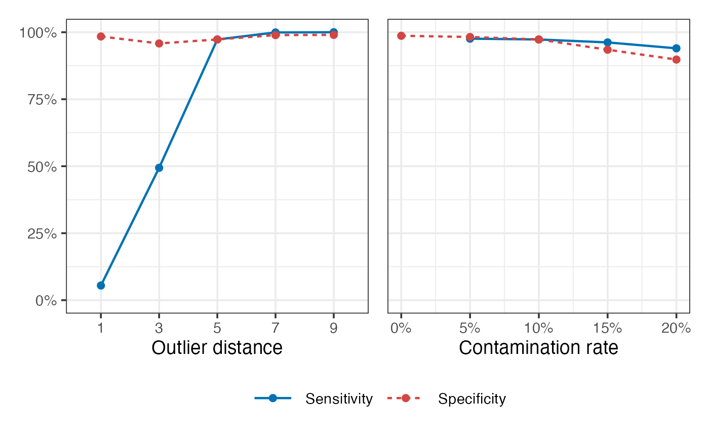

p1 = eval_metrics_study2 |> 
  filter(method == "roams_fut_model") |> 
  filter(contamination == 0.1) |> 
  pivot_longer(c(TPR, TNR), 
               names_to = "metric", values_to = "value") |> 
  mutate(metric = ifelse(metric == "TPR", "Sensitivity", "Specificity")) |> 
  ggplot() +
  aes(x = factor(distance), y = value, 
      colour = metric) +
  geom_boxplot() +
  labs(x = "Outlier distance", y = NULL, 
       colour = NULL, linetype = NULL) +
  scale_y_continuous(labels = scales::percent, limits = c(0,1)) +
  scale_colour_manual(values = c("#0072B2","#D24644FF"))

p2 = eval_metrics_study2 |> 
  filter(method == "roams_fut_model") |> 
  filter(distance == 5) |> 
  pivot_longer(c(TPR, TNR), 
               names_to = "metric", values_to = "value") |>
  mutate(metric = ifelse(metric == "TPR", "Sensitivity", "Specificity")) |> 
  ggplot() +
  aes(x = contamination, y = value,
      colour = metric, group = interaction(contamination, metric)) +
  geom_boxplot() +
  labs(x = "Contamination rate", y = NULL, 
       colour = NULL, linetype = NULL) +
  scale_y_continuous(labels = scales::percent, limits = c(0,1)) +
  scale_x_continuous(labels = scales::percent) +
  scale_colour_manual(values = c("#0072B2","#D24644FF"))

p1 + p2 + plot_layout(ncol = 2, axes = "collect", guides = "collect")

Out-of-sample MSFE

Mean-aggregated (Figure 5 of Shankar et al. (2025)) and raw box plots of the one-step-ahead out-of-sample MSFE:

• Mean MSFE
• Raw MSFE

methods = c("roams_fut_model", "roams_kalman_model", "classical_model", "huber_model", "trimmed_model", "oracle_model")
labels = c("**ROAMS-FUT**", "**ROAMS-Kalman**", "Classical", "Huber", "Trimmed", "Oracle")
colours = c("orange", "gold", "royalblue", "brown3", "purple3", "green4")
linetypes = c("solid", "solid", "dotted", "dashed", "dashed", "dotdash")

p1 = eval_metrics_study2 |> 
  filter(contamination == 0.1) |> 
  group_by(distance, method) |> 
  summarise(MSFE = mean(MSFE)) |> 
  mutate(method = factor(method, levels = methods)) |> 
  ggplot() +
  aes(x = factor(distance), y = MSFE, 
      colour = method, linetype = method, group = method) +
  geom_line(linewidth = LW) +
  geom_point(size = PS) +
  scale_colour_manual(values = setNames(colours, methods),
                      labels = setNames(labels, methods)) +
  scale_linetype_manual(values = setNames(linetypes, methods),
                        labels = setNames(labels, methods)) +
  labs(x = "Outlier distance", y = "Mean MSFE", 
       colour = NULL, linetype = NULL) +
  theme(legend.text = element_markdown())

p2 = eval_metrics_study2 |> 
  filter(distance == 5) |> 
  group_by(contamination, method) |> 
  summarise(MSFE = mean(MSFE)) |> 
  mutate(method = factor(method, levels = methods)) |> 
  ggplot() +
  aes(x = contamination, y = MSFE, 
      colour = method, linetype = method) +
  geom_line(linewidth = LW) +
  geom_point(size = PS) +
  scale_colour_manual(values = setNames(colours, methods),
                      labels = setNames(labels, methods)) +
  scale_linetype_manual(values = setNames(linetypes, methods),
                        labels = setNames(labels, methods)) +
  labs(x = "Contamination rate", y = "Mean MSFE", 
       colour = NULL, linetype = NULL) +
  scale_x_continuous(labels = scales::percent) +
  theme(legend.text = element_markdown())

p1 + p2 + plot_layout(ncol = 2, axes = "collect", guides = "collect")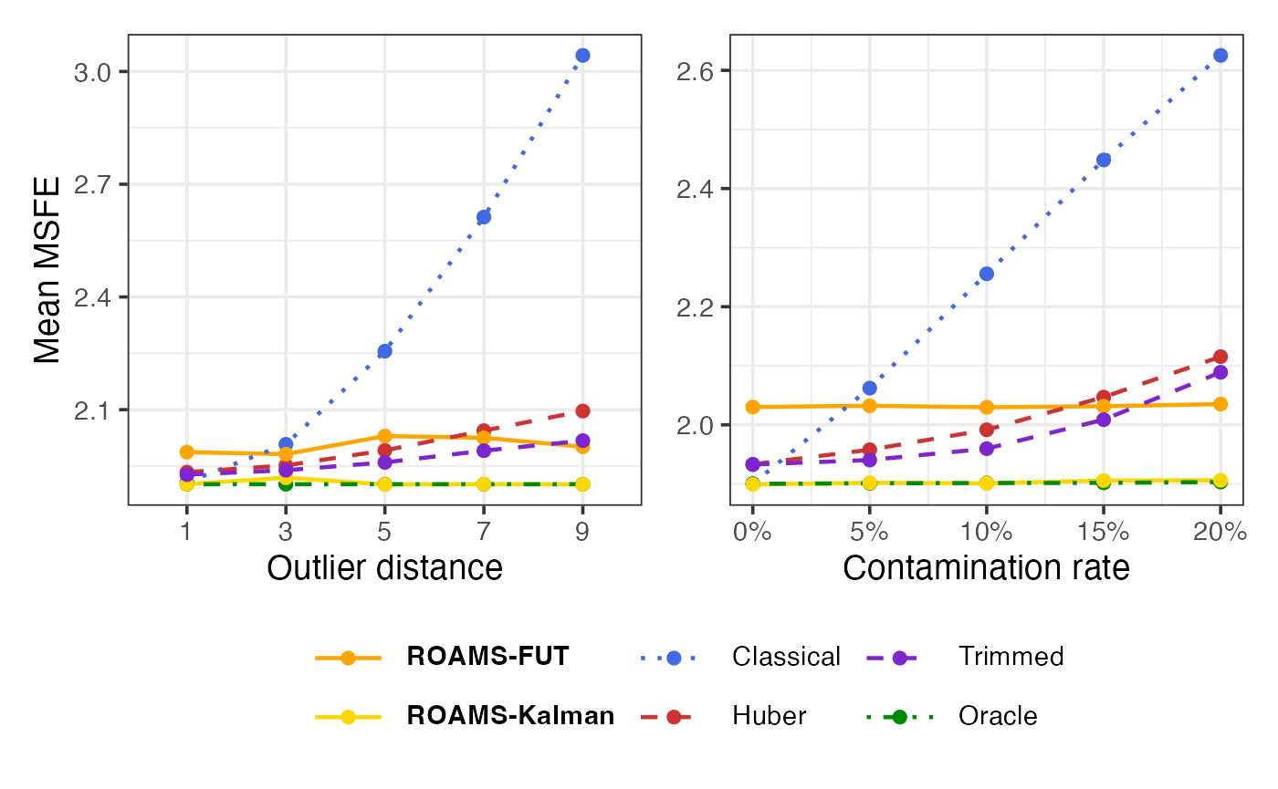

p1 = eval_metrics_study2 |> 
  filter(contamination == 0.1) |> 
  mutate(method = factor(method, levels = methods)) |> 
  ggplot() +
  aes(x = factor(distance), y = MSFE, colour = method) +
  geom_boxplot() +
  scale_colour_manual(values = setNames(colours, methods),
                      labels = setNames(labels, methods)) +
  labs(x = "Outlier distance", y = "MSFE", 
       colour = NULL) +
  theme(legend.text = element_markdown())

p2 = eval_metrics_study2 |> 
  filter(distance == 5) |> 
  mutate(method = factor(method, levels = methods)) |> 
  ggplot() +
  aes(x = contamination, y = MSFE, 
      colour = method, group = interaction(contamination, method)) +
  geom_boxplot() +
  scale_colour_manual(values = setNames(colours, methods),
                      labels = setNames(labels, methods)) +
  labs(x = "Contamination rate", y = "MSFE", 
       colour = NULL) +
  scale_x_continuous(labels = scales::percent) +
  theme(legend.text = element_markdown())

p1 + p2 + plot_layout(ncol = 2, axes = "collect", guides = "collect")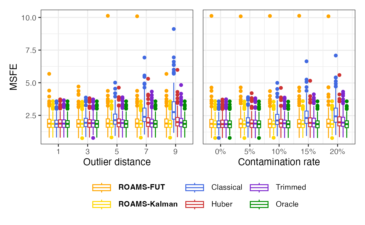

Phi: Parameter estimation error (RMSE)

Mean-aggregated and raw RMSE of each method’s phi estimate from the true value of 0.8:

• Mean RMSE
• Raw RMSE

methods = c("roams_fut_model", "classical_model", "huber_model", "trimmed_model", "oracle_model")
labels = c("**ROAMS**", "Classical", "Huber", "Trimmed", "Oracle")
colours = c("orange", "royalblue", "brown3", "purple3", "green4")
linetypes = c("solid", "dotted", "dashed", "dashed", "dotdash")

p1 = eval_metrics_study2 |> 
  filter(method != "roams_kalman_model") |> 
  filter(contamination == 0.1) |> 
  group_by(distance, method) |> 
  summarise(RMSE = mean(sqrt(par_dist_phi))) |> 
  mutate(method = factor(method, levels = methods)) |> 
  ggplot() +
  aes(x = factor(distance), y = RMSE, 
      colour = method, linetype = method, group = method) +
  geom_line(linewidth = LW) +
  geom_point(size = PS) +
  scale_colour_manual(values = setNames(colours, methods),
                      labels = setNames(labels, methods)) +
  scale_linetype_manual(values = setNames(linetypes, methods),
                        labels = setNames(labels, methods)) +
  labs(x = "Outlier distance", y = "Mean RMSE (phi)", 
       colour = NULL, linetype = NULL) +
  theme(legend.text = element_markdown())

p2 = eval_metrics_study2 |> 
  filter(method != "roams_kalman_model") |> 
  filter(distance == 5) |> 
  group_by(contamination, method) |> 
  summarise(RMSE = mean(sqrt(par_dist_phi))) |> 
  mutate(method = factor(method, levels = methods)) |> 
  ggplot() +
  aes(x = contamination, y = RMSE, 
      colour = method, linetype = method) +
  geom_line(linewidth = LW) +
  geom_point(size = PS) +
  scale_colour_manual(values = setNames(colours, methods),
                      labels = setNames(labels, methods)) +
  scale_linetype_manual(values = setNames(linetypes, methods),
                        labels = setNames(labels, methods)) +
  labs(x = "Contamination rate", y = "Mean RMSE (phi)", 
       colour = NULL, linetype = NULL) +
  scale_x_continuous(labels = scales::percent) +
  theme(legend.text = element_markdown())

p1 + p2 + plot_layout(ncol = 2, axes = "collect", guides = "collect")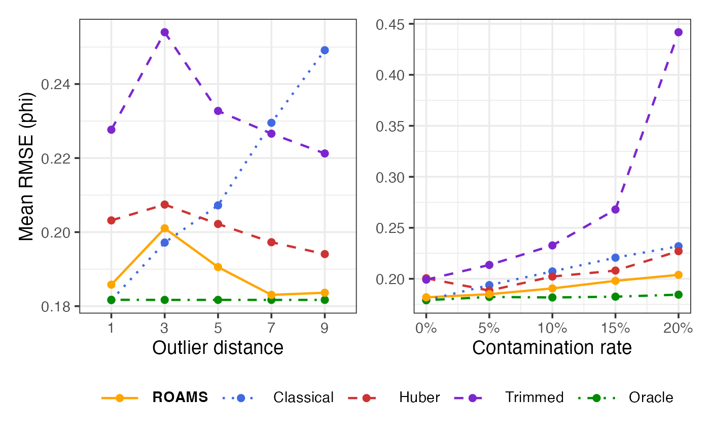

p1 = eval_metrics_study2 |> 
  filter(method != "roams_kalman_model") |> 
  filter(contamination == 0.1) |> 
  mutate(method = factor(method, levels = methods)) |> 
  ggplot() +
  aes(x = factor(distance), y = sqrt(par_dist_phi), colour = method) +
  geom_boxplot() +
  scale_colour_manual(values = setNames(colours, methods),
                      labels = setNames(labels, methods)) +
  labs(x = "Outlier distance", y = "RMSE (phi)", 
       colour = NULL) +
  theme(legend.text = element_markdown())

p2 = eval_metrics_study2 |>
  filter(method != "roams_kalman_model") |> 
  filter(distance == 5) |> 
  mutate(method = factor(method, levels = methods)) |> 
  ggplot() +
  aes(x = contamination, y = sqrt(par_dist_phi), 
      colour = method, group = interaction(contamination, method)) +
  geom_boxplot() +
  scale_colour_manual(values = setNames(colours, methods),
                      labels = setNames(labels, methods)) +
  labs(x = "Contamination rate", y = "RMSE (phi)", 
       colour = NULL) +
  scale_x_continuous(labels = scales::percent) +
  theme(legend.text = element_markdown())

p1 + p2 + plot_layout(ncol = 2, axes = "collect", guides = "collect")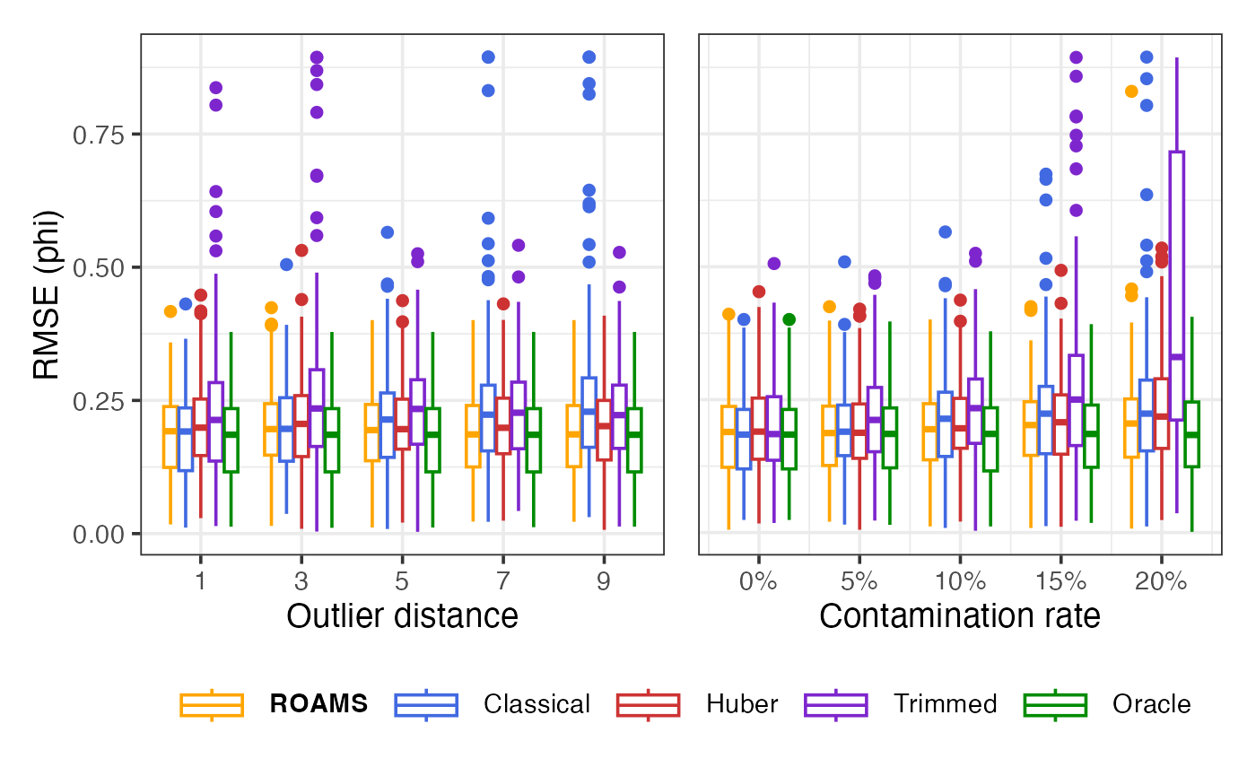

State error variances: Parameter estimation error (RMSE)

Mean-aggregated and raw RMSE of each method’s state error variances estimates from the true value of (0.1, 0.1):

• Mean RMSE
• Raw RMSE

p1 = eval_metrics_study2 |> 
  filter(method != "roams_kalman_model") |> 
  filter(contamination == 0.1) |> 
  group_by(distance, method) |> 
  summarise(RMSE = mean(sqrt(par_dist_state_var))) |> 
  mutate(method = factor(method, levels = methods)) |> 
  ggplot() +
  aes(x = factor(distance), y = RMSE, 
      colour = method, linetype = method, group = method) +
  geom_line(linewidth = LW) +
  geom_point(size = PS) +
  scale_colour_manual(values = setNames(colours, methods),
                      labels = setNames(labels, methods)) +
  scale_linetype_manual(values = setNames(linetypes, methods),
                        labels = setNames(labels, methods)) +
  labs(x = "Outlier distance", y = "Mean RMSE (state error vars)", 
       colour = NULL, linetype = NULL) +
  theme(legend.text = element_markdown())

p2 = eval_metrics_study2 |> 
  filter(method != "roams_kalman_model") |> 
  filter(distance == 5) |> 
  group_by(contamination, method) |> 
  summarise(RMSE = mean(sqrt(par_dist_state_var))) |> 
  mutate(method = factor(method, levels = methods)) |> 
  ggplot() +
  aes(x = contamination, y = RMSE, 
      colour = method, linetype = method) +
  geom_line(linewidth = LW) +
  geom_point(size = PS) +
  scale_colour_manual(values = setNames(colours, methods),
                      labels = setNames(labels, methods)) +
  scale_linetype_manual(values = setNames(linetypes, methods),
                        labels = setNames(labels, methods)) +
  labs(x = "Contamination rate", y = "Mean RMSE (state error vars)", 
       colour = NULL, linetype = NULL) +
  scale_x_continuous(labels = scales::percent) +
  theme(legend.text = element_markdown())

p1 + p2 + plot_layout(ncol = 2, axes = "collect", guides = "collect")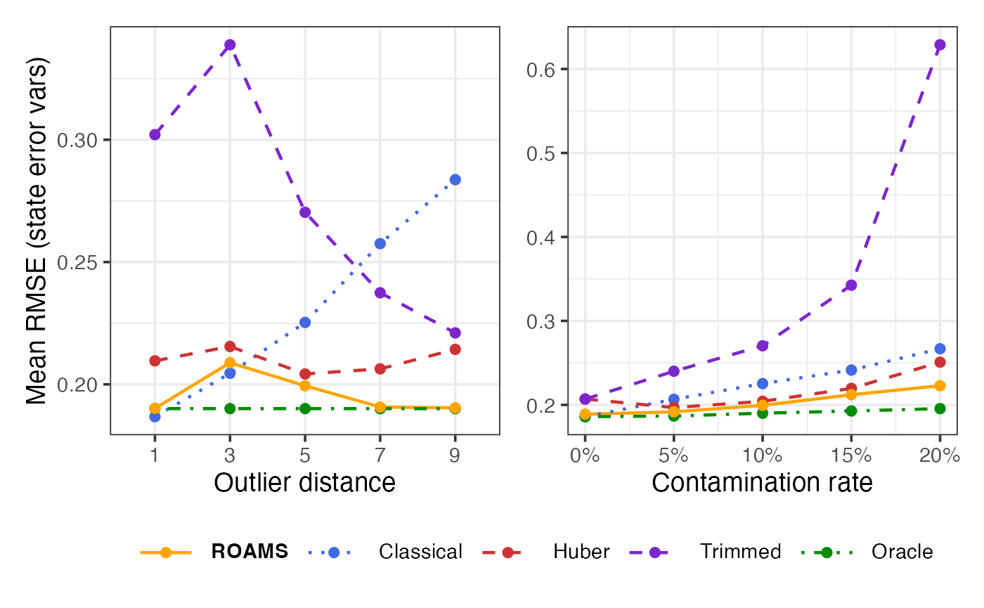

p1 = eval_metrics_study2 |> 
  filter(method != "roams_kalman_model") |> 
  filter(contamination == 0.1) |> 
  mutate(method = factor(method, levels = methods)) |> 
  ggplot() +
  aes(x = factor(distance), y = sqrt(par_dist_state_var), colour = method) +
  geom_boxplot() +
  scale_colour_manual(values = setNames(colours, methods),
                      labels = setNames(labels, methods)) +
  labs(x = "Outlier distance", y = "RMSE (state error vars)", 
       colour = NULL) +
  theme(legend.text = element_markdown())

p2 = eval_metrics_study2 |>
  filter(method != "roams_kalman_model") |> 
  filter(distance == 5) |> 
  mutate(method = factor(method, levels = methods)) |> 
  ggplot() +
  aes(x = contamination, y = sqrt(par_dist_state_var), 
      colour = method, group = interaction(contamination, method)) +
  geom_boxplot() +
  scale_colour_manual(values = setNames(colours, methods),
                      labels = setNames(labels, methods)) +
  labs(x = "Contamination rate", y = "RMSE (state error vars)", 
       colour = NULL) +
  scale_x_continuous(labels = scales::percent) +
  theme(legend.text = element_markdown())

p1 + p2 + plot_layout(ncol = 2, axes = "collect", guides = "collect")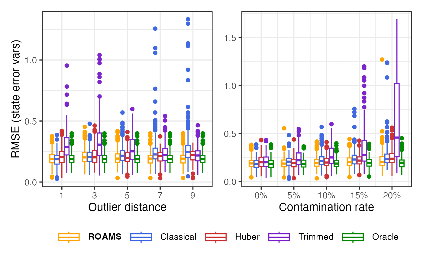

Observation error variances: Parameter estimation error (RMSE)

Mean-aggregated and raw RMSE of each method’s observation error variances estimates from the true value of (0.4, 0.4):

• Mean RMSE
• Raw RMSE

p1 = eval_metrics_study2 |> 
  filter(method != "roams_kalman_model") |> 
  filter(contamination == 0.1) |> 
  group_by(distance, method) |> 
  summarise(RMSE = mean(sqrt(par_dist_obs_var))) |> 
  mutate(method = factor(method, levels = methods)) |> 
  ggplot() +
  aes(x = factor(distance), y = RMSE, 
      colour = method, linetype = method, group = method) +
  geom_line(linewidth = LW) +
  geom_point(size = PS) +
  scale_colour_manual(values = setNames(colours, methods),
                      labels = setNames(labels, methods)) +
  scale_linetype_manual(values = setNames(linetypes, methods),
                        labels = setNames(labels, methods)) +
  labs(x = "Outlier distance", y = "Mean RMSE (obs error vars)", 
       colour = NULL, linetype = NULL) +
  theme(legend.text = element_markdown())

p2 = eval_metrics_study2 |> 
  filter(method != "roams_kalman_model") |> 
  filter(distance == 5) |> 
  group_by(contamination, method) |> 
  summarise(RMSE = mean(sqrt(par_dist_obs_var))) |> 
  mutate(method = factor(method, levels = methods)) |> 
  ggplot() +
  aes(x = contamination, y = RMSE, 
      colour = method, linetype = method) +
  geom_line(linewidth = LW) +
  geom_point(size = PS) +
  scale_colour_manual(values = setNames(colours, methods),
                      labels = setNames(labels, methods)) +
  scale_linetype_manual(values = setNames(linetypes, methods),
                        labels = setNames(labels, methods)) +
  labs(x = "Contamination rate", y = "Mean RMSE (obs error vars)", 
       colour = NULL, linetype = NULL) +
  scale_x_continuous(labels = scales::percent) +
  theme(legend.text = element_markdown())

p1 + p2 + plot_layout(ncol = 2, axes = "collect", guides = "collect")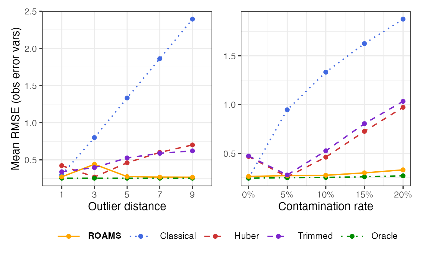

p1 = eval_metrics_study2 |> 
  filter(method != "roams_kalman_model") |> 
  filter(contamination == 0.1) |> 
  mutate(method = factor(method, levels = methods)) |> 
  ggplot() +
  aes(x = factor(distance), y = sqrt(par_dist_obs_var), colour = method) +
  geom_boxplot() +
  scale_colour_manual(values = setNames(colours, methods),
                      labels = setNames(labels, methods)) +
  labs(x = "Outlier distance", y = "RMSE (obs error vars)", 
       colour = NULL) +
  theme(legend.text = element_markdown())

p2 = eval_metrics_study2 |>
  filter(method != "roams_kalman_model") |> 
  filter(distance == 5) |> 
  mutate(method = factor(method, levels = methods)) |> 
  ggplot() +
  aes(x = contamination, y = sqrt(par_dist_obs_var), 
      colour = method, group = interaction(contamination, method)) +
  geom_boxplot() +
  scale_colour_manual(values = setNames(colours, methods),
                      labels = setNames(labels, methods)) +
  labs(x = "Contamination rate", y = "RMSE (obs error vars)", 
       colour = NULL) +
  scale_x_continuous(labels = scales::percent) +
  theme(legend.text = element_markdown())

p1 + p2 + plot_layout(ncol = 2, axes = "collect", guides = "collect")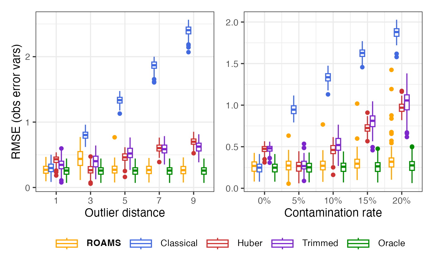

ROAMS iterations

Mean-aggregated and raw number of iterations performed by ROAMS when fitting models.

• Mean number of iterations
• Raw number of iterations

p1 = eval_metrics_study2 |> 
  filter(method == "roams_fut_model") |> 
  filter(contamination == 0.1) |> 
  group_by(distance) |> 
  summarise(iterations = mean(iterations)) |> 
  ggplot() +
  aes(x = factor(distance), y = iterations, group = 1) +
  geom_line(linewidth = LW) +
  geom_point(size = PS) +
  labs(x = "Outlier distance", y = "Mean ROAMS iterations")

p2 = eval_metrics_study2 |> 
  filter(method == "roams_fut_model") |> 
  filter(distance == 5) |> 
  group_by(contamination) |> 
  summarise(iterations = mean(iterations)) |> 
  ggplot() +
  aes(x = contamination, y = iterations) +
  geom_line(linewidth = LW) +
  geom_point(size = PS) +
  labs(x = "Contamination rate", y = "Mean ROAMS iterations") +
  scale_x_continuous(labels = scales::percent)

p1 + p2 + plot_layout(ncol = 2, axes = "collect", guides = "collect")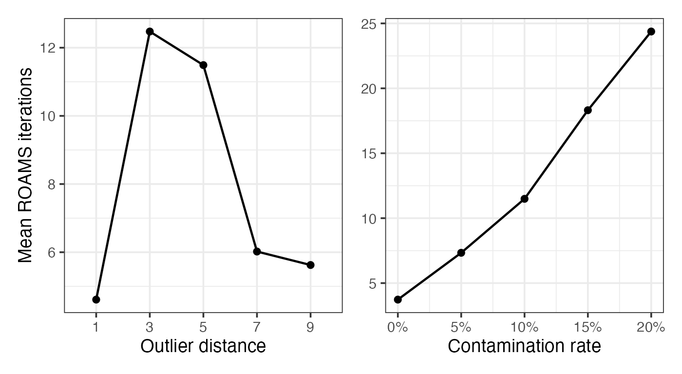

p1 = eval_metrics_study2 |> 
  filter(method == "roams_fut_model") |> 
  filter(contamination == 0.1) |> 
  ggplot() +
  aes(x = factor(distance), y = iterations) +
  geom_boxplot() +
  labs(x = "Outlier distance", y = "ROAMS iterations")

p2 = eval_metrics_study2 |> 
  filter(method == "roams_fut_model") |> 
  filter(distance == 5) |> 
  ggplot() +
  aes(x = contamination, y = iterations, group = contamination) +
  geom_boxplot() +
  labs(x = "Contamination rate", y = "ROAMS iterations") +
  scale_x_continuous(labels = scales::percent)

p1 + p2 + plot_layout(ncol = 2, axes = "collect", guides = "collect")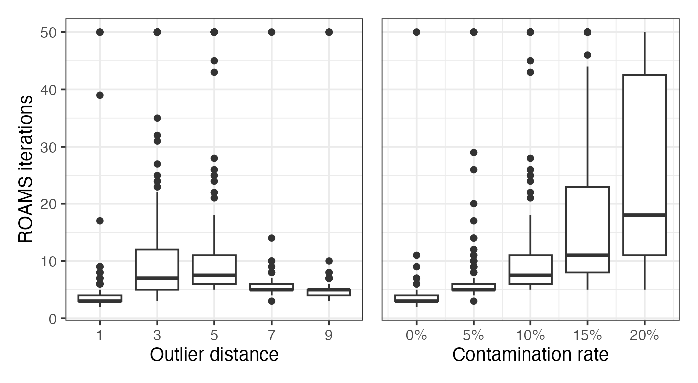

ROAMS lambda selected

Mean-aggregated and raw value of the tuning parameter $\lambda$ selected by ROAMS when fitting models.

• Mean lambda
• Raw lambda

p1 = eval_metrics_study2 |> 
  filter(method == "roams_fut_model") |> 
  filter(contamination == 0.1) |> 
  group_by(distance) |> 
  summarise(lambda = mean(lambda)) |> 
  ggplot() +
  aes(x = factor(distance), y = lambda, group = 1) +
  geom_line(linewidth = LW) +
  geom_point(size = PS) +
  labs(x = "Outlier distance", y = "Mean ROAMS lambda")

p2 = eval_metrics_study2 |> 
  filter(method == "roams_fut_model") |> 
  filter(distance == 5) |> 
  group_by(contamination) |> 
  summarise(lambda = mean(lambda)) |> 
  ggplot() +
  aes(x = contamination, y = lambda) +
  geom_line(linewidth = LW) +
  geom_point(size = PS) +
  labs(x = "Contamination rate", y = "Mean ROAMS lambda") +
  scale_x_continuous(labels = scales::percent)

p1 + p2 + plot_layout(ncol = 2, axes = "collect", guides = "collect")

p1 = eval_metrics_study2 |> 
  filter(method == "roams_fut_model") |> 
  filter(contamination == 0.1) |> 
  ggplot() +
  aes(x = factor(distance), y = lambda) +
  geom_boxplot() +
  labs(x = "Outlier distance", y = "ROAMS lambda")

p2 = eval_metrics_study2 |> 
  filter(method == "roams_fut_model") |> 
  filter(distance == 5) |> 
  ggplot() +
  aes(x = contamination, y = lambda, group = contamination) +
  geom_boxplot() +
  labs(x = "Contamination rate", y = "ROAMS lambda") +
  scale_x_continuous(labels = scales::percent)

p1 + p2 + plot_layout(ncol = 2, axes = "collect", guides = "collect")

References

Shankar, R., Wilms, I., Raymaekers, J., & Tarr, G. (2025). Robust outlier-adjusted mean-shift estimation of state-space models. https://arxiv.org/abs/????.?????